Data Warehouse Concepts

Data Warehouse:

A data warehouse is asubject-oriented, integrated, time-variant and non-volatile collection of data in support of management's decision making process.

Subject-Oriented:  A data warehouse can be used to analyze a particular subject area. For example, "sales" can be a particular subject.

Integrated: A data warehouse integrates data from multiple data sources. For example, source A and source B may have different ways of identifying a product, but in a data warehouse, there will be only a single way of identifying a product.

Time-Variant: Historical data is kept in a data warehouse. For example, one can retrieve data from 3 months, 6 months, 12 months, or even older data from a data warehouse. This contrasts with a transactions system, where often only the most recent data is kept. For example, a transaction system may hold the most recent address of a customer, where a data warehouse can hold all addresses associated with a customer.

Non-volatile: Once data is in the data warehouse, it will not change. So, historical data in a data warehouse should never be altered.

Data Warehousing:

A process of transforming data into information and making it available to users in a timely enough manner to make a difference.

 

Types of Data Warehouse

Information processing, analytical processing, and data mining are the three types of data warehouse applications that are discussed below:

• Information Processing - A data warehouse allows to process the data stored in it. The data can be processed by means of querying, basic statistical analysis, reporting using crosstabs, tables, charts, or graphs.
• Analytical Processing - A data warehouse supports analytical processing of the information stored in it. The data can be analyzed by means of basic OLAP operations, including slice-and-dice, drill down, drill up, and pivoting.
• Data Mining - Data mining supports knowledge discovery by finding hidden patterns and associations, constructing analytical models, performing classification and prediction. These mining results can be presented using the visualization tools.

Metadata

Metadata is simply defined as data about data. The data that are used to represent other data is known as metadata. For example, the index of a book serves as a metadata for the contents in the book. In other words, we can say that metadata is the summarized data that leads us to the detailed data.

In terms of data warehouse, we can define metadata as following:

• Metadata is a road-map to data warehouse.
• Metadata in data warehouse defines the warehouse objects.
• Metadata acts as a directory. This directory helps the decision support system to locate the contents of a data warehouse.

OLTP vs. OLAP:
We can divide IT systems into transactional (OLTP) and analytical (OLAP). In general we can assume that OLTP systems provide source data to data warehouses, whereas OLAP systems help to analyze it.

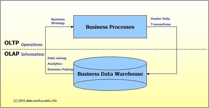
OLTP (On-line Transaction Processing) is characterized by a large number of short on-line transactions (INSERT, UPDATE, DELETE). The main emphasis for OLTP systems is put on very fast query processing, maintaining data integrity in multi-access environments and an effectiveness measured by number of transactions per second. In OLTP database there is detailed and current data, and schema used to store transactional databases is the entity model (usually 3NF). 

OLAP (On-line Analytical Processing) is characterized by relatively low volume of transactions. Queries are often very complex and involve aggregations. For OLAP systems a response time is an effectiveness measure. OLAP applications are widely used by Data Mining techniques. In OLAP database there is aggregated, historical data, stored in multi-dimensional schemas (usually star schema). 


The following table summarizes the major differences between OLTP and OLAP system design.

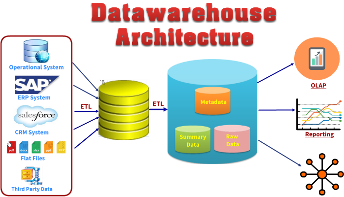
Data Warehouse Architecture:

It consists of following layers

1. Data Source layer
2. ETL
3. Staging Area
4. Data warehouse - Metadata, Summary and Raw Data
5. OLAP, Reporting and Data Mining

Data Source Layer
Data warehouse is populated from multiple sources for an organisation. All these source system comes under Data Source layer. Some of the source systems are listed below:

1. Operations Systems -- such as Sales, HR, Inventory relational database.
2. ERP (SAP) and CRM (SalesForce.com) Systems.
3. Web server logs and Internal market research data.
4. Third-party data - such as census data, demographics data, or survey data.

What is Extract, Transform and Load (ETL)?

ETL tools perform three functions to move data from one place to another:

• Extract data from sources such as ERP or CRM applications;
• Transform that data into a common format that fits with other data in the warehouse; and,
• Load the data into the data warehouse for analysis.

The ETL concept sounds easy, but the execution is complex. We’re not talking about simple copy and paste stuff here. Each step in the process has its challenges. For example, during the extract step, data may come from different source systems (e.g. Oracle, SAP, Microsoft) and different file formats such as XML, flat files with delimiters (e.g. CSV), or the worst – old legacy systems that store data in arcane formats no one else uses anymore.

The transform step may include multiple data manipulations such as splitting, translating, merging, sorting, pivoting and more. For example, a customer name might be split into first and last name, or dates might be changed to the standard ISO format (e.g. from 11-21-11 to 2011-11-21). The final step, load, involves loading the transformed data into the data warehouse. This can either be done in batch processes or row by row, more or less in real-time.

ETL tools often come bundled with databases or sold as bolt-on tools. For example, Microsoft, Oracle and IBM all offer some type of ETL capabilities with their databases. Meanwhile, third-party ETL vendors offer tools that will support a variety of disparate applications and data structures. As a final option, some BI buyers choose to build their own custom ETL tools.

We should mention that despite being a core component of data warehouse environments, ETL is not unique to data warehousing. This concept and technology has existed in some form or fashion for a long time. It can be used to move data between databases, transactional systems (e.g. ERP to CRM) and of course, data warehouses.

Staging Area
Data gets pulled from the data source into the Staging Area.This is a temporary data store area where data is pulled prior to being cleaned and transformed into a data warehouse. Having one common area makes it easier for subsequent data processing / integration.

Metadata
Metadata means data for the data. It is one of the most important aspects for data warehouse environments. Metadata helps the Business Analyst or the decision maker to find what data is in the warehouse and use that data effectively and efficiently.

Summary Data
Summary Data contains data int eh aggregated form. Data from source systems is summarized and computed as per requirements and in a way it answers specific business questions. e.g YTD , MTD, QTD information rolling over couple of years. It helps to increase the system performance by fetching data from pre computed and aggregated data.

OLAP
Online analytical processing, or OLAP is an approach to answering multi-dimensional queries in faster and quick time. OLAP tools such as Cubes, Oracle BI suite, helps users to analyze multidimensional data effectively from multiple perspectives.

OLAP consists of three basic operations: roll-up, drill-down, and slicing and dicing.

Data Mining
Data Mining is the process of discovering patterns in large data sets. The goal of the data mining process is to extract information from a data set and transform it into an understandable structure for further use. Which can be used to increase/decrease revenue, increase/descrease product supply or even cust or increase costs. It allows users to analyze data from many different dimensions or angles, categorize it, and summarize the relationships identified.

Data Modeling - Conceptual, Logical, And Physical Data Models

The three levels of data modeling, conceptual data model, logical data model, and physical data model, were discussed in prior sections. Here we compare these three types of data models. The table below compares the different features:

Feature	Conceptual	Logical	Physical
Entity Names	✓	✓
Entity Relationships	✓	✓
Attributes		✓
Primary Keys		✓	✓
Foreign Keys		✓	✓
Table Names			✓
Column Names			✓
Column Data Types			✓

Below we show the conceptual, logical, and physical versions of a single data model.

Conceptual Model Design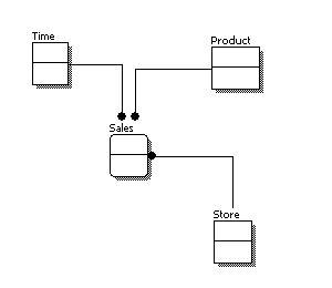

Logical Model Design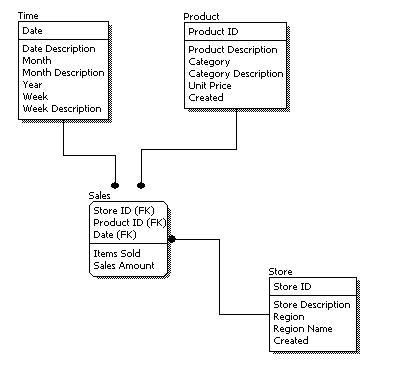

Physical Model Design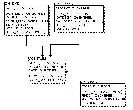

Conceptual Data Modeling:

A conceptual data model identifies the highest-level relationships between the different entities. Features of conceptual data model include:

• Includes the important entities and the relationships among them.
• No attribute is specified.
• No primary key is specified.

Logical Data Model:

A logical data model describes the data in as much detail as possible, without regard to how they will be physical implemented in the database. 

The steps for designing the logical data model are as follows:

1. Specify primary keys for all entities.
2. Find the relationships between different entities.
3. Find all attributes for each entity.
4. Resolve many-to-many relationships.
5. Normalization.

Physical Data Model:

Physical data model represents how the model will be built in the database. A physical database model shows all table structures, including column name, column data type, column constraints, primary key, foreign key, and relationships between tables. 

The steps for physical data model design are as follows:

1. Convert entities into tables.
2. Convert relationships into foreign keys.
3. Convert attributes into columns.
4. Modify the physical data model based on physical constraints / requirements.

Fact Tables and Types:

                        A fact table is the one which consists of the measurements, metrics or facts of business process. These measurable facts are used to know the business value and to forecast the future business. The different types of facts are explained in detail below.

Measure types

Fact table can store different types of measures such as additive, non-additive, semi additive.

Additive:

            Additive facts are facts that can be summed up through all of the dimensions in the fact table. A sales fact is the best example for additive fact.

Semi Additive:

            Semi additive are the fact tables that can be summed up for some of the dimensions in the fact table, but not the others.

Eg: Daily balances fact can be summed up through the customer dimension but not through the time dimension.

Non Additive:

            Non additive facts are fact tables that cannot be summed up for any of the dimensions present in the fact table.

Eg: Facts with have percentages, ratios calculated.

Factless Fact table:

            In the real world it is possible to have fact table that contains no measures or facts. These tables are called factless fact tables.

Eg: A fact table which has only product key and date key is a factless fact. There are no measures in this table. But still you can get the number products sold over a period of time.

A fact tables that contain aggregated facts are often called summary tables. 

Types of fact tables:

All fact tables are categorized by three most basic measurement events:

• Transactional – Transactional fact table is the most basic one that each grain associated with it indicated as “one row per line in a transaction”, e.g., every line item appears on an invoice. Transaction fact table stores data of the most detailed level therefore it has high number of dimensions associated with.

• Periodic snapshots – Periodic snapshots fact table stores data that is a snapshot in a period of time. The source data of periodic snapshots fact table is data from a transaction fact table where you choose period to get the output.

• Accumulating snapshots – The accumulating snapshots fact table describes activity of a business process that has clear beginning and end. This type of fact table therefore has multiple date columns to represent milestones in the process. A good example of accumulating snapshots fact table is processing of a material. As steps towards handling the material are finished, the corresponding record in the accumulating snapshots fact table get updated.

 Dimensions Tables:

A dimension table consists of the attributes about the facts. Dimensions store the textual /descriptions of the business attribute. Without the dimensions, we cannot measure the facts and facts are just disordered Numbers. In Business, Customer, Products, Buyers information can be different dimensions.

Let’s walk through commonly used types of dimensions.

• Conformed Dimensions
• Junk Dimensions
• Role-playing Dimensions
• Slowly Changing Dimensions
• Degenerated Dimensions

Conformed Dimensions:

A Dimension that is used in multiple locations is called conformed dimensions. A conformed dimension may be used with multiple fact tables in single database, or across multiple data marts or Data warehouses.

I.e. Above shown Customer and Product Dimensions are Conformed Dimensions as they are connected to Shipment Fact table, Sales Order Fact table, and Service Request Fact table.

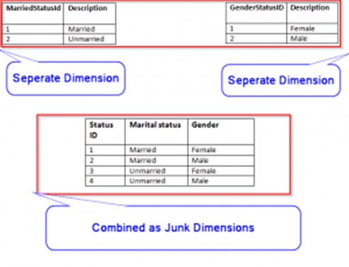
Junk Dimensions

A junk dimension is a collection of random transaction codes flags and/or text attributes that are unrelated to any particular dimension. The junk dimension is simply a structure that provides a convenient place to store the junk attributes.

I.e.:  Assume that we have a gender dimension and marital status dimension. In the fact table we need to maintain two keys referring to these dimensions. Instead of that create a junk dimension which has all the combinations of gender and marital status (cross join gender and marital status table and create a junk table). Now we can maintain only one key in the fact table.

Role-playing Dimensions

A role-playing dimension is one where the same dimension key — along with its associated attributes — can be joined to more than one foreign key in the fact table. For example, a fact table may include foreign keys for both Ship Date and Delivery Date. But the same date dimension attributes apply to each foreign key, so you can join the same dimension table to both foreign keys. Here the date dimension is taking multiple roles to map ship date as well as delivery date, and hence the name of Role Playing dimension.

I.e.:  In Date dimensions, [FullDateAlternateKey] is associated with [Orderdate key], [Duedate key], and [Shipdate] key in the fact table to solve different purpose in Data warehouse.

Slowly Changing Dimensions

This is widely used Dimensions type. It is the dimensions where attribute values changes with time. There are various types of Slowly Changing Dimensions (SCD) based on how business manages this dimensions.

Types of SCD

TYPE 0: It is the dimensions where we do not change attribute values at all. They are rarely used. I.e. Employee birth date

TYPE 1: In this type, Old value of attribute is overwritten by new values of attribute and no history kept

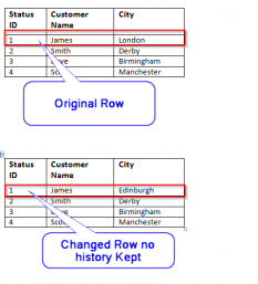
I.e Customer City where company decided to show only current one.

In this case previous city name London is replaced by new city name Edinburgh.

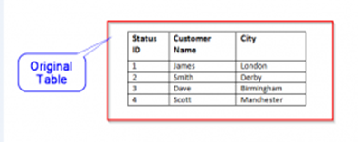
TYPE 2: In this type we tracks historical data by creating multiple records for a given Natural key (business key) in the dimensional tables with separate surrogate key and/or different version numbers. Unlimited history is preserved for each insert.

I.e. Customer City where company decided to have historical data then we will have to add an extra row with column to identify the Current/Historical attributes value by start and end date columns.

TYPE 3: In this type, we tracks changes using separate columns and preserves limited history.it is limited to how many columns we want to add in dimension table.

I.e. Customer City where New columns “previous City” and “Current City” being added.

TYPE 4: In this type, we keep all or some historical data in separate table and current data stays in main Dimension table. Both historical and current dimension table joined to fact table with same surrogate key, this will enhance the query performance. This type    used very rarely.

 

I.e. we create new table to store previous Customer City and Current Customer City in Historical table with Created date And Current Customer city in Current dimension table.

Degenerated Dimensions:

A degenerate dimension is when the dimension attribute is stored as part of fact table, and not in a separate dimension table. These are essentially dimension keys for which there are no other attributes. In a data warehouse, these are often used as the result of a drill through query to analyze the source of an aggregated number in a report. You can use these values to trace back to transactions in the OLTP system.

I.e. Invoice no can be stored in the fact table and then used as separate dimensions for the drill through purpose to find out what invoices are part of total buying cost in report.

So Dimensions are one of the pillar of the data warehouse. Choosing right one can define future of the data warehouse. It always good to use right type

Hope this post gives some insight and information around data warehouse design.

Has anyone came across Rapidly Changing Dimensions??

Any suggestion and/or comment always welcome.

In the next post,I will walk through  Different Types of Facts and Fact tables.

DW Dimensional Modeling : Types of schemas

            There are four types of schemas are available in data warehouse. Out of which the star schema is mostly used in the data warehouse designs. The second mostly used data warehouse schema is snow flake schema.

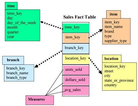
Star Schema:
            A star schema is the one in which a central fact table is surrounded by de-normalized dimensional tables. A star schema can be simple or complex. A simple star schema consists of one fact table where as a complex star schema have more than one fact table.

Snow Flake Schema:
            Snow flake schema is an enhancement of star schema by adding additional dimensions. Snow flake schema are useful when there are low cardinality attributes in the dimensions.

Galaxy Schema:
            Galaxy schema contains many fact tables with some common dimensions (conformed dimensions). This schema is a combination of many data marts.

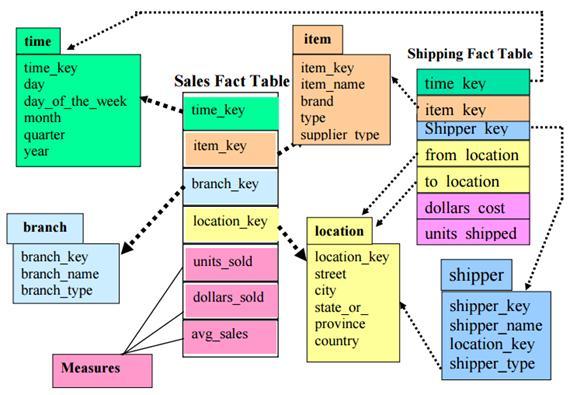
Fact Constellation Schema:
            The dimensions in this schema are segregated into independent dimensions based on the levels of hierarchy. For example, if geography has five levels of hierarchy like teritary, region, country, state and city; constellation schema would have five dimensions instead of one. 

Schema Definition:

Multidimensional schema is defined using Data Mining Query Language (DMQL). The two primitives, cube definition and dimension definition, can be used for defining the data warehouses and data marts.

Syntax for Cube Definition

define cube < cube_name > [ < dimension-list > }: < measure_list >

Syntax for Dimension Definition

define dimension < dimension_name > as ( < attribute_or_dimension_list > )

Star Schema Definition:

The star schema that we have discussed can be defined using Data Mining Query Language (DMQL) as follows:

define cube sales star [time, item, branch, location]:   

      

dollars sold = sum(sales in dollars), units sold = count(*)      

define dimension time as (time key, day, day of week, month, quarter, year)

define dimension item as (item key, item name, brand, type, supplier type)        

define dimension branch as (branch key, branch name, branch type)              

define dimension location as (location key, street, city, province or state, country)

Snowflake Schema Definition:

Snowflake schema can be defined using DMQL as follows:

define cube sales snowflake [time, item, branch, location]:

dollars sold = sum(sales in dollars), units sold = count(*)

define dimension time as (time key, day, day of week, month, quarter, year)

define dimension item as (item key, item name, brand, type, supplier (supplier key, supplier type))

define dimension branch as (branch key, branch name, branch type)

define dimension location as (location key, street, city (city key, city, province or state, country))

Fact Constellation Schema Definition:

Fact constellation schema can be defined using DMQL as follows:

define cube sales [time, item, branch, location]:

dollars sold = sum(sales in dollars), units sold = count(*)

define dimension time as (time key, day, day of week, month, quarter, year)

define dimension item as (item key, item name, brand, type, supplier type)

define dimension branch as (branch key, branch name, branch type)

define dimension location as (location key, street, city, province or state,country)

define cube shipping [time, item, shipper, from location, to location]:

dollars cost = sum(cost in dollars), units shipped = count(*)

define dimension time as time in cube sales

define dimension item as item in cube sales

define dimension shipper as (shipper key, shipper name, location as location in cube sales, shipper type)

define dimension from location as location in cube sales

define dimension to location as location in cube sales